Customer Segmentation & Causal Targeting
An end-to-end analysis on the public Dunnhumby retail dataset — NMF + K-Means segmentation feeding meta-learner / Causal-Forest HTE and an OPE-validated targeting policy.
⏱️ TL;DR (30 seconds)
- Problem — Whom should we send the coupon campaign (TypeA) to? Sending to everyone only inflates cost and produces a loss.
- Approach — A 2-Track Framework. Track 1 answers “who are our customers?” (NMF + K-Means → 7 segments); Track 2 answers “whom should we target?” (CATE estimation → policy learning).
- Three key results
- High-value segments (VIP Heavy, Bulk Shoppers) show a counter-intuitively negative (-) CATE → ceiling / cannibalization effect.
- Targeting only 31.3% (152/486) of the cohort under a CATE > breakeven ($42.43) rule is profit-optimal.
- The observational data exhibits a severe positivity violation (PS AUC = 0.989, overlap 17%) → results are hypothesis-generating and require confirmation via an A/B test.
- Impact in one line — Optimal targeting (+$2,426) versus targeting everyone (-$4,659) yields a +$7,085 / +200pp ROI improvement (on the analysis cohort; hypothesis-generating estimate).
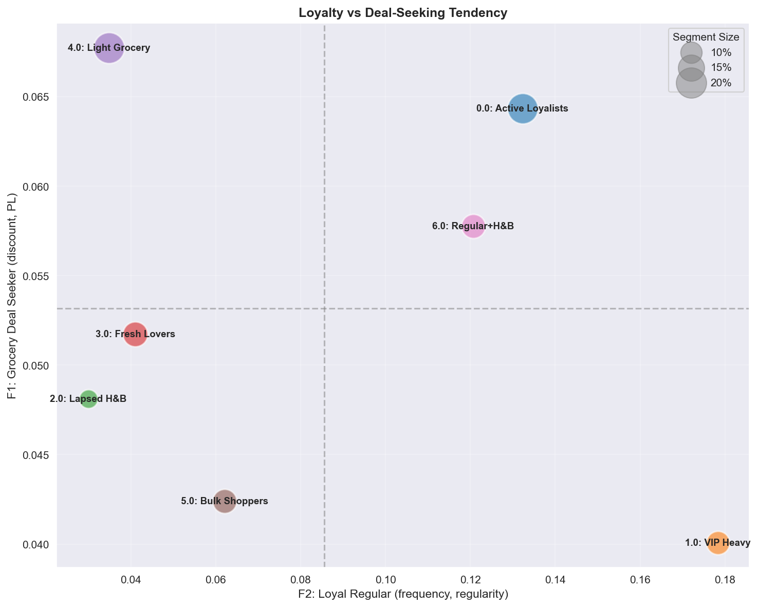 Track 1 — seven behavioral segments in loyalty (F2) × deal-seeking (F1) space.
 Track 2 — ROI peaks near ~31% targeting; targeting everyone loses money.
🎯 Key Results at a Glance
| Key metric | Value | Notes |
|---|---|---|
| Data scale | 2,500 households · ~2.6M transactions · 102 weeks | Dunnhumby “The Complete Journey” |
| Number of segments | 7 (NMF k=5 → K-Means k=7) | 92.44% variance explained, bootstrap ARI 0.77±0.11 |
| Breakeven CATE | $42.43 | cost $12.73 / margin 0.30 |
| Optimal targeting | 31.3% (152 / 486) | profit +$2,426, ROI 125% |
| Target everyone (100%) | 486 customers | profit -$4,659, ROI -75% |
| Current practice (62.1%) | 302 customers | profit -$3,402, ROI -88% |
| Improvement (optimal vs. all) | +$7,085 | +200pp ROI (hypothesis-generating) |
| Positivity diagnostic | PS AUC 0.989, overlap 17% | severe violation → hypothesis-generating reading |
| Primary CATE model | CausalForestDML | chosen on low-variance/validity grounds (see Track 2 for details) |
CATE by segment — the negative effect of high-value segments is the counter-intuitive crux
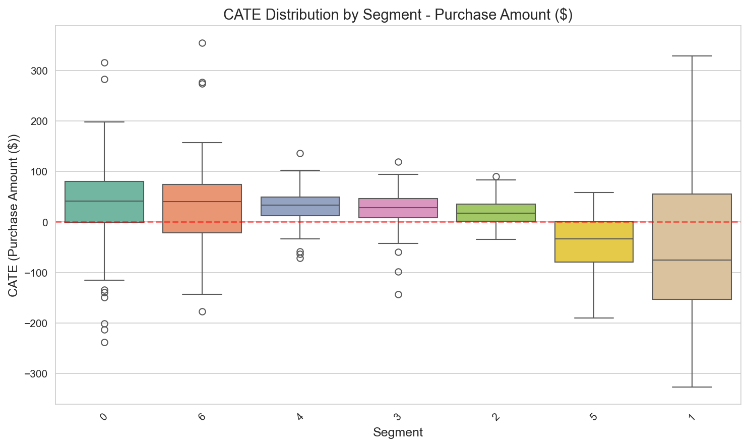 CATE distribution by segment. The negative effects of VIP Heavy (-$38) and Bulk Shoppers (-$40) are clear — a signal to scale targeting down.
Motivation & Framework
This project tackles, within a single pipeline, both the traditional segmentation question “who are our customers?” and the causal-inference question “for whom, and by how much, is this campaign effective?”.

Why are both tracks needed?
| Aspect | Track 1 (Descriptive) | Track 2 (Causal) |
|---|---|---|
| Core question | ”Who is this customer?" | "Will the campaign be effective for this customer?” |
| Main users | Marketing, CRM, Strategy | Data Science, Optimization |
| Explainability | ”Premium Fresh Lover segment" | "This customer’s CATE = +$34” |
| Organizational requirement | Marketing capability grounded in customer understanding | Causal thinking + an execution framework for personalized targeting |
Key Insights: Counter-Intuitive Findings
Negative (-) Treatment Effect of High-Value Customers
The N values below are based on the Track 2 analysis cohort (486 customers) and differ from Track 1’s full segment sizes (509, 299, …). CATE is a hypothesis-generating estimate.
| Segment | Customer value (overall mean revenue) | Mean CATE | N (cohort) | Direction signal |
|---|---|---|---|---|
| VIP Heavy | $9,716 (highest) | -$38 | 59 | Scale down / exclude from TypeA |
| Bulk Shoppers | $3,206 | -$40 | 77 | Scale down / exclude from TypeA |
Why do high-value customers show a negative CATE?
| Segment | Root-cause analysis |
|---|---|
| VIP Heavy | Already a high purchaser → ceiling effect; the coupon merely substitutes for existing purchases (cannibalization) |
| Bulk Shoppers | Coupon-based TypeA mismatches their irregular, bulk-buying shopping rhythm |
Business impact (on the 486-customer analysis cohort; hypothesis-generating):

Results Summary
Track 1 Results: Latent Factor Modeling + Clustering
Interpretation of the 5 latent factors (NMF k=5, 92.44% variance explained):
| Factor | Name | Top features (loading) | Interpretation |
|---|---|---|---|
| F1 | Grocery Deal Seeker | share_grocery(6.72), discount_usage_pct(5.13), private_label_ratio(3.41) | Discount-seeking, budget-conscious |
| F2 | Loyal Regular | purchase_regularity(4.63), n_departments(2.61), n_products(1.53), frequency(1.04) | One-stop, high-engagement (Value) |
| F3 | Big Basket | monetary_std(2.45), monetary_avg_basket(2.35), share_grocery(2.08) | Irregular bulk purchases (Value) |
| F4 | Fresh Focused | share_fresh(2.26), n_departments(1.21) | Fresh-food specialist (Need) |
| F5 | Health & Beauty | share_health_beauty(2.03), recency(0.41) | Drugstore type (Need) |
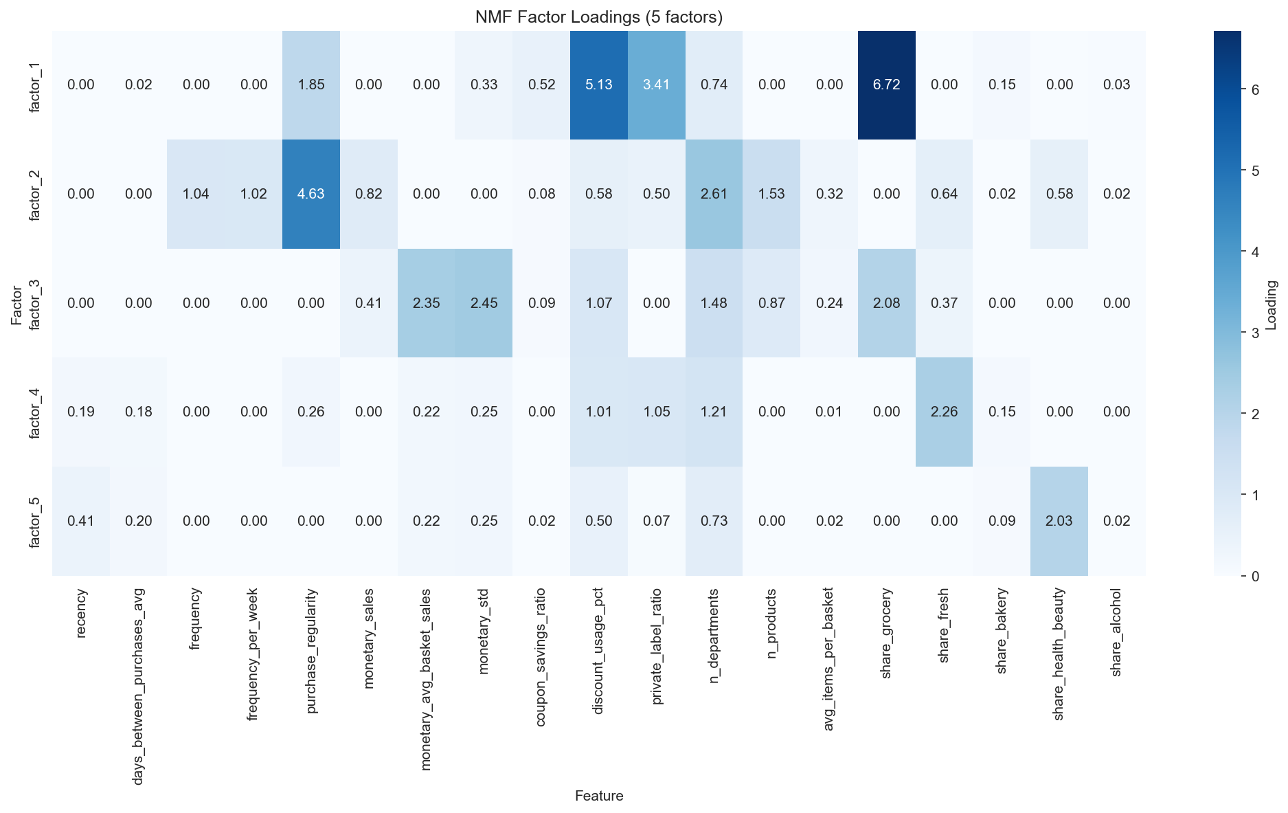 Feature loadings of the 5 latent factors. F2 (Loyal) and F3 (Big Basket) capture the Value dimension; F4 (Fresh) and F5 (H&B) capture the Need dimension.
Clustering evaluation metrics (summary):
| Metric | Value | Interpretation |
|---|---|---|
| Explained Variance | 92.44% | High factor coverage |
| Silhouette Score (k=7) | 0.219 | Reasonable for behavioral data (not the global maximum — see appendix) |
| Calinski-Harabasz (k=7) | 732.0 | — |
| Davies-Bouldin Index (k=7) | 1.241 | Minimum among k candidates (best separation) |
| Bootstrap ARI | 0.77 ± 0.11 (n=100) | High segment stability |
Honest rationale for choosing k: Silhouette is in fact highest at low k (k=3 = 0.271). k=7 was chosen on the grounds of minimum DBI (1.241) + business interpretability/actionability + high bootstrap stability (ARI 0.77). We do not claim that “silhouette is highest at k=7.” (Full grid in the Track 1 report appendix.)
The 7 customer segments (based on all 2,500 customers):
| Seg | Name | Size | Mean revenue | Frequency (visits) | Recency (days) | Regularity | Main factor |
|---|---|---|---|---|---|---|---|
| 0 | Active Loyalists | 509 (20.4%) | $3,878 | 171 | 6 | 0.78 | F2 (Loyal) |
| 1 | VIP Heavy | 299 (12.0%) | $9,716 | 256 | 4 | 0.88 | F2 (Loyal) |
| 2 | Lapsed H&B | 193 (7.7%) | $872 | 37 | 75 | 0.25 | F5 (H&B) |
| 3 | Fresh Lovers | 339 (13.6%) | $1,233 | 48 | 36 | 0.34 | F4 (Fresh) |
| 4 | Light Grocery | 524 (21.0%) | $942 | 43 | 42 | 0.30 | F1 (Grocery-Deal) |
| 5 | Bulk Shoppers | 318 (12.7%) | $3,206 | 56 | 24 | 0.41 | F3 (Basket) |
| 6 | Regular + H&B | 318 (12.7%) | $3,393 | 152 | 12 | 0.70 | F2 (Loyal) |
Light Grocery (Seg 4) has its grocery share (0.56) + discount (0.51) loading onto F1 (Grocery-Deal), so its main factor is recorded as F1.
 The seven segments in loyalty (F2) × deal-seeking (F1) space. VIP Heavy (high-loyalty / low-deal = premium) and Active Loyalists (high-loyalty / high-deal = budget-conscious loyal) respond to discounts in opposite ways despite both being “loyal” — this positioning gap is the behavioral basis for the per-segment CATE split in Track 2.
Marketing strategy by segment (Track 1 based):
| Segment | Priority | Strategy | Key actions |
|---|---|---|---|
| VIP Heavy | High | Retention | Premium benefits, churn prediction, exclusive access |
| Active Loyalists | High | Strengthen | Private-label promotions, loyalty points, basket expansion |
| Regular + H&B | Medium | Upgrade | VIP-conversion program, cross-category incentives |
| Bulk Shoppers | Medium | Regularize | Subscription offers, scheduled delivery, bundle deals |
| Fresh Lovers | Medium | Engage | Fresh-food content, daily specials, recipes |
| Light Grocery | Low | Activate | Habit-forming campaigns, gradual rewards |
| Lapsed H&B | Low | Win-back | Re-engagement campaigns, H&B-focused offers |
💡 Track 1 vs. Track 2 strategy difference: Track 1 is a general strategy based on customer characteristics; Track 2 is a TypeA-campaign targeting strategy based on CATE. VIP Heavy is “Retention” in Track 1, but in Track 2 it diverges into a recommendation to “scale down” TypeA targeting.
Track 2 Results: CATE and Optimal Targeting
ATE estimation (by method, n=2,430):
| Method | ATE | 95% CI | Reliability |
|---|---|---|---|
| Naive | +$471 | [$442, $501] | ❌ Upward bias |
| IPW | +$151 | [-$10, $313] | ⚠️ Unstable |
| AIPW | +$24 | [-$56, $104] | ✅ Doubly-robust |
| OLS | +$65 | [$29, $102] | — |
| DML | -$65 | [-$220, $90] | ⚠️ Direction reversal |
| ATO (Overlap) | +$60 | [-$14, $134] | ✅ Overlap-focused |
The estimates scatter widely across methods, from -$65 to +$471 — a direct symptom of the positivity violation. We place more trust in the overlap-focused estimate (ATO +$60) and the doubly-robust estimate (AIPW +$24).
CATE model performance (main run; test set):
| Model | Mean CATE | Test Std | AUUC | % positive | Selection |
|---|---|---|---|---|---|
| CausalForestDML | +$15 | $52 | 271.6 | 78% | ✅ Primary |
| LinearDML | -$139 | $452 | 357.0 | 42% | ❌ Highest AUUC but unstable |
| NonParamDML | +$1.1M (diverges) | very large | 304.4 | 64% | ❌ Diverges |
| S-Learner | -$21 | $46 | 289.5 | 21% | ❌ 79% negative effects (unrealistic) |
| X-Learner | -$96 | $208 | 218.5 | 38% | ❌ High variance |
| T-Learner | -$200 | $397 | 212.0 | 43% | ❌ High variance |
Model-selection rationale (honest reframe): CausalForestDML does not have the highest AUUC. In the main run the highest AUUC belongs to LinearDML (357.0), with CausalForestDML in 4th place (271.6). We nonetheless chose CausalForestDML as the primary model because it is the only model that simultaneously satisfies low variance (std $52 vs. LinearDML’s $452) and a valid CATE distribution (mean +$10–15, 78% positive — consistent with the campaign’s objective). The models with higher AUUC are unusable: LinearDML (mean -$139, std $452), NonParamDML (diverges); S-Learner has similar variance but implies an unrealistic distribution in which 79% of customers have a negative effect. Under a severe positivity violation, stability and validity take priority over raw AUUC. (Supporting evidence: BLP test p=0.094 borderline, X-Learner p=0.005 — the heterogeneity signal is weak. See the Track 2 report for details.) For the full cohort (486 customers), CausalForestDML’s mean CATE is consistently +$10.
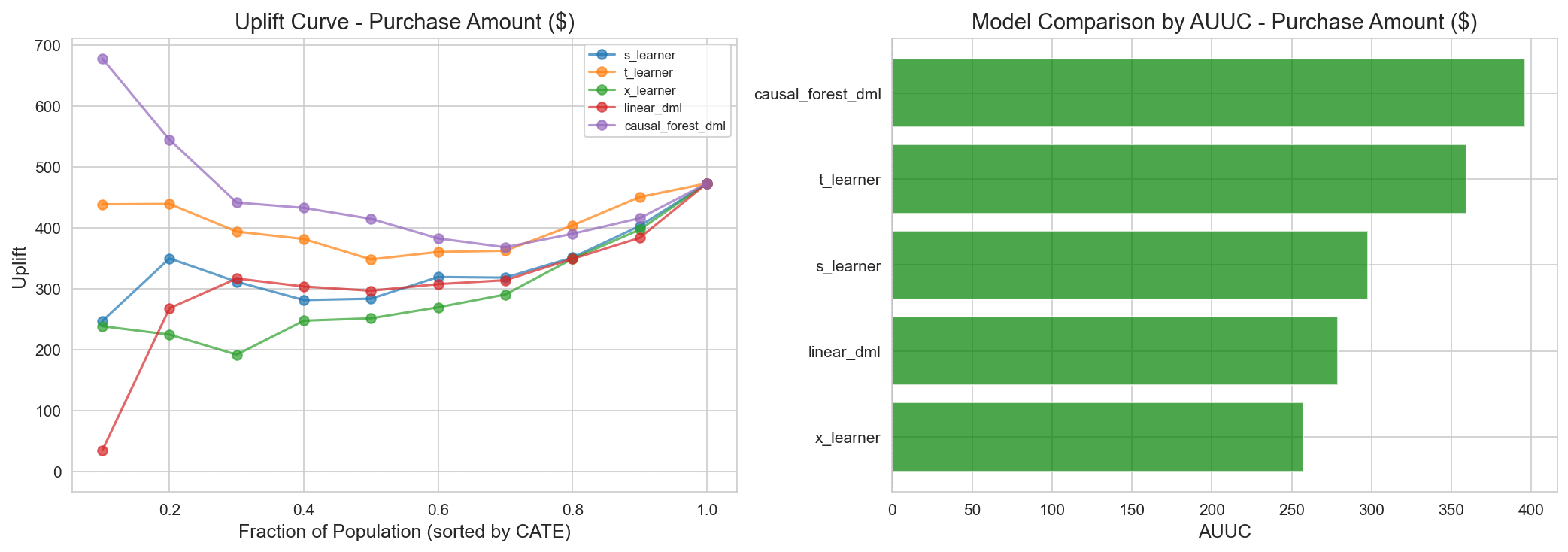 AUUC comparison across CATE models. The uplift curve of CausalForestDML, selected on stability/validity grounds. Targeting the top 30% is expected to yield $2,200+ in additional revenue.
CATE and Recommended Action by Segment
N is based on the Track 2 analysis cohort (486 customers) and differs from Track 1’s full segment sizes. “Current/recommended targeting %” is not a value present in the source CSV, so it is presented only as a direction (expand/hold/scale down).
| Segment | N (cohort) | Mean CATE | Recommended action (direction) |
|---|---|---|---|
| Active Loyalists | 97 | +$33 | Test & Learn (slight expand) |
| Regular + H&B | 62 | +$34 | Test & Learn (slight expand) |
| Light Grocery | 91 | +$30 | Test & Learn (expand) |
| Fresh Lovers | 73 | +$27 | Test & Learn (expand) |
| Lapsed H&B | 27 | +$19 | Test & Learn |
| VIP Heavy | 59 | -$38 | Scale down / exclude from TypeA |
| Bulk Shoppers | 77 | -$40 | Scale down / exclude from TypeA |
CATE distribution by segment. The negative effects of VIP Heavy (-$38) and Bulk Shoppers (-$40) are clear.
Policy Comparison Analysis (486-customer cohort)
| Policy | Criterion | Target % (N) | Profit | ROI | Characteristic |
|---|---|---|---|---|---|
| CATE > Breakeven | Point est. > $42.43 | 31.3% (152) | +$2,426 | 125% | ✅ Optimal |
| Top 20% CATE | Percentile | 20.0% (97) | +$2,259 | 183% | Highest ROI under budget constraint |
| Conservative | Lower CI > $42.43 | 0.6% (3) | +$188 | 493% | Ultra-conservative (pre-A/B) |
| Risk-Adjusted (30%) | Risk-adjusted | 11.1% (54) | +$1,603 | 233% | Variance penalty |
| PolicyTree (Tuned) | Learned rule | 26.7% (130) | +$1,684 | 102% | Interpretable |
| CATE > 0 | Point est. > 0 | 64.6% (314) | +$1,447 | 36% | Loose rule |
| Current practice | — | 62.1% (302) | -$3,402 | -88% | ❌ Loss |
| Target everyone | — | 100% (486) | -$4,659 | -75% | ❌ Loss |
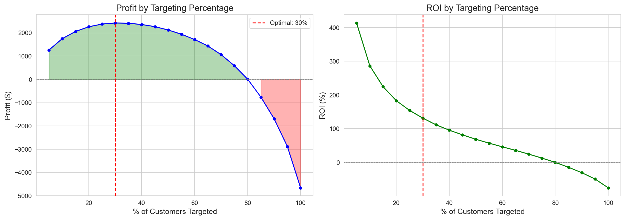 Targeting customers from the highest CATE downward, ROI peaks near 31% (+$2,426 / 125%) and then bends as negative-CATE customers accumulate, turning into a loss (−$4,659) at 100% targeting — one chart showing that whom you exclude matters as much as whom you include.
Limitations & Lessons Learned
| Limitation | Evidence | Mitigation |
|---|---|---|
| Positivity Violation | PS AUC = 0.989, overlap 17% | PS trimming, ATO weighting, Manski bounds, partial identification |
| Refutation Test failures | Placebo (Amount) 0.747 (>0.5 → FAIL), Subset Stability 0.561 (<0.7 → FAIL) | A/B test validation design (n=5,748) |
| Model disagreement | CausalForest +$10 vs. LinearDML -$139 | Selection on stability/validity grounds; acknowledge directional disagreement |
| Single campaign type | Only TypeA analyzed | TypeB/C require separate analysis |
Refutation failed — and that is the expected result. Placebo Treatment (Amount) = 0.747 (threshold <0.5) and Subset Stability = 0.561 (threshold >0.7) both failed to pass their thresholds (though Placebo-Visits = 0.052 passed). This is the expected signal under a positivity violation, and it supports treating the results as hypothesis-generating rather than confirmatory. The results are neither hidden nor softened.
Lessons
“PS AUC 0.989 reveals the fundamental limit of an observational study. The results should be interpreted as hypothesis-generating, and deployed only after validation via an A/B test.”
Future Directions
- A/B test validation: validate the hypotheses with n=5,748 (2,874/arm, 80% power, α=0.05, detectable effect ~$34).
- ε-greedy exploration: assign treatment to every customer with at least probability ε → guarantees positivity.
- MLOps extension: a CATE monitoring dashboard and a model-retraining pipeline.